What will you find in this repository?

I have two main objectives:

• demystify PySpark's partitioning techniques for reading data concurrently from a Relational Database and why data skewed and low cardinality columns should be avoided
• talk about how I've managed to improve the performance of my queries in a production Amazon EMR environment and decrease the execution time with more than 95%, by replacing Panda's read_sql() with PySpark's JDBC functionality

I've also written an article about this topic on Medium.

How can you improve the execution time of a query with more than 95%?

This is a fair question. You don't read everyday about 95% improvements in a project by just changing one library with another, but there is a reason why 80% of the Fortune 500 companies use Apache Spark (source: https://spark.apache.org/).

Apache Spark is a multi-language engine for executing data engineering, data science, and machine learning on single-node machines or clusters. It is a powerful tool for big data processing, but it can also be used to access data stored in databases. In this repo, I will show you how to use Spark’s JDBC read option to access data from a database in a distributed fashion, as well as why Pandas falls short when trying to execute an SQL query that returns millions of records.

Pandas example:

The syntax for executing SQL queries in Pandas is pretty straightforward. You need a Connection object that contains your host, port, user, password, database name and depending on your environment, ssl set to True. Some other options can be passed as well to this object but for the purpose of this example, I won't explore them.

Executing a generic SQL query in a Vertica database using Pandas and passing the mandatory arguments stored as environment variables looks like this:

query = 'SELECT f1, f2, f3 FROM table'
conn_info = {
    'host': os.environ["host"],
    'port': os.environ["port"],
    'user': os.environ["user"],
    'password': os.environ["pass"],
    'database': os.environ["db_name"],
    'ssl': True,
}

with vertica_python.connect(**conn_info) as connection:
    df = pd.read_sql(query, con=connection)

PySpark example:

The PySpark syntax is a little bit more complex, but the performance gains are so high that it's difficult making a convincing case for not using it. Let's see how it looks, following the same example as above (Vertica database, environment variables):

query = 'SELECT f1, f2, f3 FROM table'
partitionsCount = 50

df = spark.read \
    .format("jdbc") \
    .option("driver", "com.vertica.jdbc.Driver") \
    .option("url", f"jdbc:vertica://{os.environ["host"]}:{os.environ["port"]}") \
    .option("user", os.environ['user']) \
    .option("password", os.environ['pass']) \
    .option("ssl", "True") \
    .option("sslmode", "require") \
    .option("dbtable", query) \
    .option("numPartitions", partitionsCount) \
    .option("partitionColumn", "date") \
    .option("lowerBound", f"{min_date}") \
    .option("upperBound", f"{max_date}") \
    .load()

So why is Pandas not the best choice to execute a query that returns millions of rows?

It's pretty simple: Pandas has been designed to be highly optimized for single-threaded data processing. Pandas creator (Wes McKinney) said that he was not thinking about analyzing 100GB or 1TB datasets when he built Pandas. Trying to use Pandas with large datasets (or trying to load millions of rows through read_sql() is not and will never be a great experience.

What about Spark?

Configuring it properly, Spark will execute the SQL query concurrently. I'm highlighting 'properly' because not passing the correct arguments will just make the Spark task use a single executor core and at that point you're just swapping Pandas w/ Spark without any performance gains. More details about this below:

When transferring large amounts of data between Spark and an external RDBMS by default JDBC data sources loads data sequentially using a single executor thread, which can significantly slow down your application performance, and potentially exhaust the resources of your source system. In order to read data concurrently, the Spark JDBC data source must be configured with appropriate partitioning information so that it can issue multiple concurrent queries to the external database. source: https://luminousmen.com/post/spark-tips-optimizing-jdbc-data-source-reads

Let's talk about numPartitions, partitionColumn, lowerBound and upperBound:

I won't go into details about the first 8 options since they are self explanatory (if not, Spark's official documentation might be a good read: https://spark.apache.org/docs/latest/sql-data-sources-jdbc.html). But I'm going to explain the last four, since these options are the ones that make the magic happen 🙂

• numPartitions: The maximum number of partitions that can be used for parallelism in table reading. This also determines the maximum number of concurrent JDBC connections. The correct number of partitions depends on the memory assigned to your executor instances (JVM instances), how large is your dataset, and how many executor cores (number of slots available to run tasks in parallel) you have set up in your Spark Session. Keep in mind that Spark assigns one task per partition, so each partition will be processed by one executor core.
• These options describe how to partition the table when reading in parallel from multiple workers:
  • partitionColumn: partitionColumn must be a numeric, date, or timestamp column from the table in question. For the best possible performance, the column values must be as evenly distributed as possible and have high cardinality. Avoid data skewness. And using an indexed column will bring even more performance gains.
  • lowerBound, upperBound: Notice that lowerBound and upperBound are just used to decide the partition stride, not for filtering the rows in table. All rows in the table will be partitioned and returned.
• What if we don’t know upfront the lower and upper bounds of our column?
  • This is a good example where we can use Pandas to identify the lowerBound and upperBound through Pandas. Once we know that, we can pass the results as arguments to the Spark lower/upper bound parameters.

  min_max_query = f"SELECT min(date), max(date) from ({query}) as q"
  df_min_max = pd.read_sql(min_max_query, con=connection)
  min_date = df_min_max['min'].dt.date.values[0]
  max_date = df_min_max['max'].dt.date.values[0]
  

• What if we don’t have any numeric, date, or timestamp column, or it has skewed data?
  • Not a problem. We know SQL, so using a CTE and one Window Function to generate a numeric column through the row_number() function should be a piece of cake:

  with cte as
  (
      SELECT f1, f2, f3
      FROM table
  )
  select *, row_number() over (order by f1) as rn from cte
  

Why data skewed columns should be avoided?

Let’s imagine we have a dataset w/ 20M rows and 30 partitions, lower and upper bound being 2020-01-01 and 2022-12-31 (I will talk in more detail about lowerbound and upperbound below. For now, just know that these bounds don't filter the data but they define how the data will be read and partitioned in the Spark dataframe). For the purpose of the presentation, we’ll use a Spark Session with 30 executor cores (we can run up to 30 tasks at the same time). Keep in mind that Spark assigns one task per partition, so each partition will be processed by one executor core.

Each year worth of data will be divided in 10 partitions and considering that 1 task will be assigned to 1 partition, each task assigned to years 2020 and 2021 will be responsible for processing 100k rows, but each task assigned to year 2022 will have to process 1.8M rows. That’s a 1700% increase in data that must be processed by one task.

The result is that the first 20 tasks will finish processing their assigned partition in no time and after that the 20 executor cores assigned to the completed tasks will sit idle until the last 10 tasks finish processing 1700% more records. This is a waste of resources and increase in operating costs, especially if you use Spark in an EMR cluster, Glue Job, or Databricks.

How do we fix that? There are two things we can do: we can either use a different column for partitioning the data, or if it's critical to use this column, we create two queries and two dataframes instead of one. The first query will load the first two years (the 30 executor cores will be divided between year 2020 and 2021), then the second query will load the final year (so all the 30 executor cores will be used for year 2022). Because of that, one task from year 2022 will now be responsible for processing 600k instead of 1.8M rows. That's a 66% decrease in rows that must be processed by a single executor core and on top of that, we now use all the executor cores from our Spark Session instead of having them sit idle.

Why low cardinality columns should be avoided?

(photo source: https://luminousmen.com/)

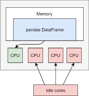
Imagine that the column you want to use for partitioning has only `0` and `1` values - an extreme example indeed, but a common scenarion where boolean values `True` and `False` are converted to numeric values. Based on how the partitions are generated - see the above picture - all the rows with the value `0` will be pushed to the first partition and all the rows with the value `1` will be pushed to the last partition. So, regardless of how many partitions you want to create, only two partitions will be populated and only two executor cores will do all the work, the other ones will be in an idle state. Because of that, the performance of the executed query will suffer dramatically.